About ELEKTRONN2¶

Introduction
Design principles
- Nodes and layers
- Network models
Features
Documentation and usage examples
Contributors
License

Introduction ¶

What is ELEKTRONN2?¶

ELEKTRONN2 is a flexible and extensible Python toolkit that facilitates design, training and application of neural networks.

It can be used for general machine learning tasks, but its main focus is on convolutional neural networks (CNNs) for high-throughput 3D and 2D image analysis.

ELEKTRONN2 is especially useful for efficiently assessing experimental neural network architectures thanks to its powerful interactive shell that can be entered at any time during training, temporarily pausing all calculations.

The shell interface provides shortcuts and autocompletions for frequently used operations (e.g. adjusting the learning rate) and also provides a complete python shell with full read/write access to the network model, the plotting subsystem and all training parameters and hyperparameters. Changes made in the shell take effect immediately, so you can monitor, analyse and manipulate your training sessions directly during their run time, without losing any training progress.

Computationally expensive calculations are automatically compiled and transparently executed as highly-optimized CUDA binaries on your GPU if a CUDA-compatible graphics card is available [1].

ELEKTRONN2 is written in Python (2.7 / and 3.4+) and is a complete rewrite of the previously published ELEKTRONN library. The largest improvement is the development of a functional interface that allows easy creation of complex data-flow graphs with loops between arbitrary points in contrast to simple “chain”-like models. Currently, the only supported platform is Linux (x86_64).

[1]	You can find out if your graphics card is compatible here. Usage on systems without CUDA is possible but generally not recommended because it is very slow.

Use cases ¶

Although other high-level libraries are available (Keras, Lasagne), they all lacked desired features and flexibility for our work, mostly in terms of an intuitive method to specify complicated computational graphs and utilities for training and data handling, especially in the domain of specialised large-scale 3-dimensional image data analysis for connectomics research (e.g. tracing, mapping and segmenting neurons in in SBEM [2] data sets).

Although the mentioned use cases are ELEKTRONN2’s specialty, it can be used and extended for a wide range of other tasks thanks to its modular object-oriented API design (for example, new operations can be implemented as subclasses of the Node class and seamlessly integrated into neural network models).

[2]	Serial Block-Face Scanning Electron Microscopy, a method to generate high resolution 3D images from small samples, such as brain tissue.

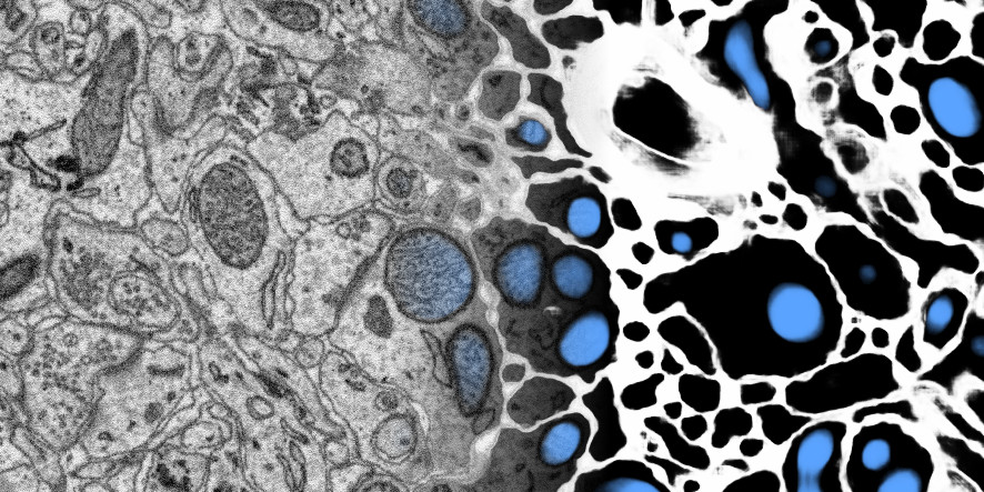
Example visualisation of ELEKTRONN2’s usage on a 3D SBEM data set (blending input to output from left to right).

Left (input: raw data)	Right (output: predictions by ELEKTRONN2, color-coded)
3D electron microscopy images of a zebra finch brain (area X dataset j0126 by Jörgen Kornfeld).	Probability of barriers (union of cell boundaries and extracellular space, marked in white) and mitochondria (marked in blue) predicted by ELEKTRONN2.

Technology ¶

As the back-end we chose Theano because of good prior experience and competitive performance. With Theano, symbolic computational graphs can be created, in which nodes stand for operations and edges carry values (input and output can be seen as a special operation i.e. a node). Theano is able to compile a graph into a binary executable for different targets (CPU, openMP, GPUs with CUDA support); highly optimised routines from numerical libraries for those targets (e.g. BLAS, cuBLAS, cuDNN) will be used for corresponding operations. Using a symbolic graph facilitates automatic differentiation and optimisation of the graph prior to compilation (e.g. common subexpression elimination, fusion of composed element-wise operations, constant folding). For (convolutional) neural networks the GPU is the most efficient target and Theano can itself be seen as a back-end for low-level CUDA.

Other dependencies:

matplotlib (plotting of training statistics and prediction previews)
h5py (reading and writing data sets)
numpy (math and data types)
scipy (math and image handling)
numba (accelerating numpy code)
future (maintaining Python 2/3 compatibility)
tqdm (progress bars in the CLI)
colorlog (logging framework)
prompt_toolkit (interactive training shell)
jedi (shell autocompletions)
scikit-learn (cross-validation)
scikit-image (image processing)
seaborn (plot style)
pydotplus (visualizing computation graphs)
psutil (parallelisation)

Design principles ¶

ELEKTRONN2 adds another abstraction layer to Theano. To create a model, the user has to connect different types of node objects and thereby builds a graph as with Theano. But the creation of the raw Theano graph, composed of symbolic variables and trainable model parameters, is hidden and managed through usage of sensible default values and bundling of stereotypical Theano operations into a single ELEKTRONN2 node. For example, creating a convolution layer consists of initialising weights, performing the convolution, adding the bias, applying the activation function and optional operations such as dropout or batch normalisation. Involved parameters might be trainable (e.g. convolution weights) or non-trainable but changeable during training (e.g. dropout rates).

Nodes and layers ¶

Nodes automatically keep track of their parents and children, parameters, computational cost, output shape, spatial field of view, spatial strides etc. Users can call a node object simply like a numpy function. The corresponding Theano compilation is done on demand upon first call; all arguments Theano needs for the compilation process are automatically gathered from the node meta data. Methods for profiling, checking the correct output shape or making dense predictions with a (strided) CNN on arbitrarily shaped input are additionally provided. Shapes are augmented with usage tags e.g. ‘x’, ‘y’, ‘z’ for spatial axes, ‘f’ for the feature axis.

Nodes are mostly generic, e.g. the Perceptron node can operate on any input by reading from the input shape tags which axis the dot product should be applied over, irrespective of the total input dimensionality. Likewise there is only one type of convolution node which can handle 1-, 2- and 3-dimensional convolutions and determines the case based on the input shape tags, it does also make replacements of the convolution operation if this makes computation faster: for a 3-dimensional convolution where the filter size is 1 on the z-axis using a 2-dimensional convolution back-end is faster for gradient computation; convolutions where all filter shapes are 1 can be calculated faster using the dot product.

Network models ¶

Whenever a Node is created, it is registered internally to a model object which also records the exact arguments with which the node was created as node descriptors. The model provides an interface for the trainer by designating nodes as input, target, loss and monitoring outputs. The model also offers functions for plotting the computational graph as image, and showing statistics about gradients, neuron activations and parameters (mean, standard deviation, median).

Furthermore, the model offers methods loading and saving from/to disk. Because for this the descriptors are used and not the objects itself, these can programmatically be manipulated before restoration of a saved graph. This is used for: * changing input image size of a CNN (including sanity check of new shape), * inserting Max-Fragment-Pooling (MFP) into a CNN that was trained without MFP, * marking specific parameters as non-trainable for faster training, * changing batch normalisation from training mode to prediction mode * creating a one-step function from a multi-step RNN.

Features ¶

Operations ¶

Perceptron / fully-connected / dot-product layer, works for arbitrary dimensional input
Convolution, 1-,2-,3-dimensional
Max/Average Pooling, 1,2,3-dimensional
UpConv, 1,2,3-dimensional
Max Fragment Pooling (MFP), 1,2,3-dimensional
Gated Recurrent Unit (GRU) and Long Short Term Memory (LSTM) unit
Recurrence / Scan over arbitrary sub-graph: support of multiple inputs multiple outputs and feed-back of multiple values per iteration
Batch normalisation with automatic accumulation of whole data set statistics during training
Gaussian noise layer (for Variational Auto Encoders)
Activation functions: tanh, sigmoid, relu, prelu, abs, softplus, maxout, softmax-layer
Local Response Normalisation (LRN), feature-wise or spatially
Basic operations such as concatenation, slicing, cropping, or element-wise functions

Loss functions ¶

Bernoulli / Multinoulli negative log likelihood
Gaussian negative log likelihood
Squared Deviation Loss, (margin optional)
Absolute Deviation Loss, (margin optional)
Weighted sum of losses for multi-task training

Optimisers ¶

Stochastic Gradient Descent (SGD)
AdaGrad
AdaDelta
Adam

Trainer ¶

Automatic creation of training directory to which all files (parameters, log files, previews etc.) will be saved
Frequent printing and logging of current state, iteration speed etc.
Frequent plotting of monitored states (error samples on training and validation data, classification errors and custom monitoring targets)
Frequent saving of intermediate parameter states and history of monitored variables
Frequent preview prediction images for CNN training
Customisable schedules for non-trainable meta-parameters (e.g. dropout rates, learning rate, momentum)
Fully functional python command line during training, usable for debugging/inspection (e.g. of inputs, gradient statistics) or for changing meta-parameters

Training Examples for CNNs ¶

Randomised patch extraction from a list of of input/target image pairs
Data augmentation trough histogram distortions, rotation, shear, stretch, reflection and perspective distortion
Real-time data augmentation through a queue with background threads.

Utilities ¶

Array interface for KNOSSOS data sets with caching, pre-fetching and support for multiple data sets as channel axis.
Viewer for multichannel 3-dimensional image arrays within the Python runtime
Function to convert ID images to boundary images
Utilities needed for skeltonisation agent training and application
Visualisation of the computational graph
Class for profiling within loops
KD Tree that supports append (realised through mixture of KD-Tree and brute-force search and amortised rebuilds)
Daemon script for the synchronised start of experiments on several hosts, based on resource occupation.