Examples¶

This page gives examples for different use cases of ELEKTRONN2. Besides, the examples are intended to give an idea of how custom network architectures could be created and trained without the built-in pipeline. To understand the examples, basic knowledge of neural networks is recommended.

3D CNN architecture and concepts
- Defining the neural network model
- Exploring Model and Node objects
3D Neuro Data (examples/neuro3d.py)

3D CNN architecture and concepts ¶

Here we explain how a simple 3-dimensional CNN and its loss function can be specified in ELEKTRONN2. The model batch size is 10 and the CNN takes an [23, 183, 183] image volume with 3 channels [1] (e.g. RGB colours) as input.

[1]	For consistency reasons the axis containing image channels and the axis containing classification targets are also denoted by `'f'` like the feature maps or features of a MLP.

Defining the neural network model ¶

The following code snippet [2] exemplifies how a 3-dimensional CNN model can be built using ELEKTRONN2.

[2]	For complete network config files that you can directly run with little to no modification, see the 3d Neuro Data section below and the “examples” directory in the code repository, especially neuro3d.py.

# The neuromancer submodule contains the API to define neural network models.
# It is usually accessed via the alias "nm".
from elektronn2 import neuromancer as nm

# Input shape: (batch size, number of features/channels, z, x, y)
image = nm.Input((10, 3, 23, 183, 183), 'b,f,z,x,y', name='image')

# If no node name is given, default names and enumeration are used.
# 3d convolution with 32 filters of size (1,6,6) and max-pool sizes (1,2,2).
# Node constructors always receive their parent node as the first argument
# (except for the root nodes like the 'image' node here).
conv0 = nm.Conv(image, 32, (1,6,6), (1,2,2))
conv1 = nm.Conv(conv0, 64, (4,6,6), (2,2,2))
conv2 = nm.Conv(conv1, 5, (3,3,3), (1,1,1), activation_func='lin')

# Softmax automatically infers from the input's 'f' axis
# that the number of classes is 5 and the axis index is 1.
class_probs = nm.Softmax(conv2)

# This copies shape and strides from class_probs but the feature axis
# is overridden to 1, the target array has only one feature on this axis,
# the class IDs i.e. 'sparse' labels. It is also possible to use 5
# features where each contains the probability for the corresponding class.
target = nm.Input_like(class_probs, override_f=1, name='target', dtype='int16')

# Voxel-wise loss calculation
voxel_loss = nm.MultinoulliNLL(class_probs, target, target_is_sparse=True)
scalar_loss = nm.AggregateLoss(voxel_loss , name='loss')

# Takes class with largest predicted probability and calculates classification accuracy.
errors = nm.Errors(class_probs, target, target_is_sparse=True)

# Creation of nodes has been tracked and they were associated to a model object.
model = nm.model_manager.getmodel()

# Tell the model which nodes fulfill which roles.
# Intermediates nodes like conv1 do not need to be explicitly registered
# because they only have to be known by their children.
model.designate_nodes(
    input_node=image,
    target_node=target,
    loss_node=scalar_loss,
    prediction_node=class_probs,
    prediction_ext=[scalar_loss, errors, class_probs]
)

model.designate_nodes() triggers printing of aggregated model stats and extended shape properties of the prediction_node.
Executing the above model creation code prints basic information for each node and its output shape and saves it to the log file.
Example output:

<Input-Node> 'image'
Out:[(10,b), (3,f), (23,z), (183,x), (183,y)]
---------------------------------------------------------------------------------------
<Conv-Node> 'conv'
#Params=3,488 Comp.Cost=25.2 Giga Ops, Out:[(10,b), (32,f), (23,z), (89,x), (89,y)]
n_f=32, 3d conv, kernel=(1, 6, 6), pool=(1, 2, 2), act='relu',
---------------------------------------------------------------------------------------
<Conv-Node> 'conv1'
#Params=294,976 Comp.Cost=416.2 Giga Ops, Out:[(10,b), (64,f), (10,z), (42,x), (42,y)]
n_f=64, 3d conv, kernel=(4, 6, 6), pool=(2, 2, 2), act='relu',
---------------------------------------------------------------------------------------
<Conv-Node> 'conv2'
#Params=8,645 Comp.Cost=1.1 Giga Ops, Out:[(10,b), (5,f), (8,z), (40,x), (40,y)]
n_f=5, 3d conv, kernel=(3, 3, 3), pool=(1, 1, 1), act='lin',
---------------------------------------------------------------------------------------
<Softmax-Node> 'softmax'
Comp.Cost=640.0 kilo Ops, Out:[(10,b), (5,f), (8,z), (40,x), (40,y)]
---------------------------------------------------------------------------------------
<Input-Node> 'target'
Out:[(10,b), (1,f), (8,z), (40,x), (40,y)]
85
---------------------------------------------------------------------------------------
<MultinoulliNLL-Node> 'nll'
Comp.Cost=640.0 kilo Ops, Out:[(10,b), (1,f), (8,z), (40,x), (40,y)]
Order of sources=['image', 'target'],
---------------------------------------------------------------------------------------
<AggregateLoss-Node> 'loss'
Comp.Cost=128.0 kilo Ops, Out:[(1,f)]
Order of sources=['image', 'target'],
---------------------------------------------------------------------------------------
<_Errors-Node> 'errors'
Comp.Cost=128.0 kilo Ops, Out:[(1,f)]
Order of sources=['image', 'target'],
Prediction properties:
[(10,b), (5,f), (8,z), (40,x), (40,y)]
fov=[9, 27, 27], offsets=[4, 13, 13], strides=[2 4 4], spatial shape=[8, 40, 40]
Total Computational Cost of Model: 442.5 Giga Ops
Total number of trainable parameters: 307,109.
Computational Cost per pixel: 34.6 Mega Ops

Exploring `Model` and `Node` objects ¶

The central concept in ELEKTRONN2 is that a neural network is represented as a Graph of executable Node objects that are registered and organised in a Model.

In general, we have one Model instance that is called model by convention (see elektronn2.neuromancer.model.Model.

All other variables here are instances of different subclasses of Node, which are implemented in the neuromancer.node_basic, neuromancer.neural, neuromancer.loss and neuromancer.various submodules.

For more detailed information about Node and how its subclasses are derived, see the Node API docs.

After executing the above code (e.g. by %paste-ing into an ipython session or by running the whole file via elektronn2-train and hitting Ctrl+C during training), you can play around with the variables defined there to better understand how they work.

Node objects can be used like functions to calculate their output.
The first call triggers compilation and caches the compiled function:

>>> import numpy as np
>>> test_input = np.ones(shape=image.shape.shape, dtype=np.float32)
>>> test_output = class_probs(test_input)
Compiling softmax, inputs=[image]
Compiling done - in 21.32 s
>>> np.all(test_output > 0) and np.all(test_output < 1)
True

The model object has a dict interface to its Nodes:

>>> model
['image', 'conv', 'conv1', 'conv2', 'softmax', 'target', 'nll', 'loss', 'cls for errors', 'errors']
>>> model['nll'] == voxel_loss
True
>>> conv2.shape.ext_repr
'[(10,b), (5,f), (8,z), (40,x), (40,y)]\nfov=[9, 27, 27], offsets=[4, 13, 13],
strides=[2 4 4], spatial shape=[8, 40, 40]'
>>> target.measure_exectime(n_samples=5, n_warmup=4)
Compiling target, inputs=[target]
Compiling done - in 0.65 s
86
target samples in ms:
[ 0.019 0.019 0.019 0.019 0.019]
target: median execution time: 0.01903 ms

For efficient dense prediction, batch size is changed to 1 and MFP is inserted.
To do that, the model must be rebuilt/reloaded.
MFP needs a different patch size. The closest possible one is selected:

>>> from elektronn2 import neuromancer as nm
>>> model_prediction = nm.model.rebuild_model(model, imposed_batch_size=1,
                                                       override_mfp_to_active=True)
patch_size (23) changed to (22) (size not possible)
patch_size (183) changed to (182) (size not possible)
patch_size (183) changed to (182) (size not possible)
---------------------------------------------------------------------------------------
<Input-Node> 'image'
Out:[(1,b), (3,f), (22,z), (182,x), (182,y)]
...

Dense prediction: test_image can have any spatial shape as long as it is larger than the model patch size:

>>> model_prediction.predict_dense(test_image, pad_raw=True)
Compiling softmax, inputs=[image]
Compiling done - in 27.63 s
Predicting img (3, 58, 326, 326) in 16 Blocks: (4, 2, 2)
...

The whole model can also be plotted as a graph by using the elektronn2.utils.d3viz.visualize_model() method:

>>> from elektronn2.utils.d3viz import visualise_model
>>> visualise_model(model, '/tmp/modelgraph')

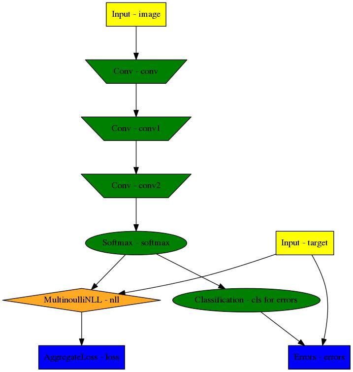
Model graph of the example CNN. Inputs are yellow and outputs are blue.
Some node classes are represented by special shapes, the default shape is oval.

3D Neuro Data (`examples/neuro3d.py`)¶

Note

This section is under construction and is currently incomplete.

In the following concrete example, ELEKTRONN2 is used for detecting neuron cell boundaries in 3D electron microscopy image volumes. The more general goal is to find a volume segmentation by assigning a cell ID to each voxel. Predicting boundaries is a surrogate target for which a CNN can be trained. The actual segmentation would be made by e.g. running a watershed transformation on the predicted boundary map. This is a typical img-img task.

For demonstration purposes, a relatively small CNN with only 3M parameters and 7 layers is used. It trains fast but is obviously limited in accuracy. To solve this task well, more training data would be required in addition.

The full configuration file on which this section is based can be found in ELEKTRONN2’s examples folder as neuro3d.py. If your GPU is slow or you want to try ELEKTRONN2 on your CPU, we recommend you use the neuro3d_lite.py config instead. It uses the same data and has the same output format, but it runs significantly faster (at the cost of accuracy).

Getting Started ¶

Download and unpack the neuro_data_zxy test data (98 MiB):

wget http://elektronn.org/downloads/neuro_data_zxy.zip
unzip neuro_data_zxy.zip -d ~/neuro_data_zxy

cd to the examples directory or download the example file to your working directory:

wget https://raw.githubusercontent.com/ELEKTRONN/ELEKTRONN2/master/examples/neuro3d.py

Run:
```
elektronn2-train neuro3d.py --gpu=auto
```

During training, you can pause the neural network and enter the interactive shell interface by pressing Ctrl+C. There you can directly inspect and modify all (hyper-)parameters and options of the training session.

Inspect the printed output and the plots in the save directory
You can start experimenting with changes in the config file (for example by inserting a new Conv layer) and validate your model by directly running the config file through your Python interpreter before trying to train it:
```
python neuro3d.py
```

Data Set ¶

This data set is a subset of the zebra finch area X dataset j0126 by Jörgen Kornfeld. There are 3 volumes which contain “barrier” labels (union of cell boundaries and extra cellular space) of shape (150,150,150) in (z,x,y) axis order. Correspondingly, there are 3 volumes which contain raw electron microscopy images. Because a CNN can only make predictions within some offset from the input image extent, the size of the image cubes is larger (250,350,350) in order to be able to make predictions and to train for every labelled voxel. The margin in this examples allows to make predictions for the labelled region with a maximal field of view of 201 in x, y and 101 in z.

There is a difference in the lateral dimensions and in z - direction because this data set is anisotropic: lateral voxels have a spacing of $10 \mu m$ in contrast to $20 \mu m$ vertically. Snapshots of images and labels are depicted below.

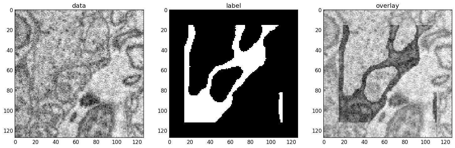
An example slice of the neuro_data_zxy data set

Left	Center	Right
Raw input data	Barrier labels	Labels overlayed on top of input data.

During training, the pipeline cuts image and target patches from the loaded data cubes at randomly sampled locations and feeds them to the CNN. Therefore the CNN input size should be smaller than the size of the data cubes, to leave enough space to cut from many different positions. Otherwise it will always use the same patch (more or less) and soon over-fit to that one.

During training initialisation a debug plot of a randomly sampled batch is made to check whether the training data is presented to the CNN in the intended way and to find errors (e.g. image and label cubes are not matching or labels are shifted w.r.t. images). Once the training loop has started, more such plots can be made from the ELEKTRONN2 command line (Ctrl+C)

>>> mfk@ELEKTRONN2: self.debug_getcnnbatch()

Note

Implementation details: When the cubes are read into the pipeline, it is implicitly assumed that the smaller label cube is spatially centered w.r.t the larger image cube (hence the size surplus of the image cube must be even). Furthermore, for performance reasons the cubes are internally zero-padded to the same size and cropped such that only the area in which labels and images are both available after considering the CNN offset is used. If labels cannot be effectively used for training (because either the image surplus is too small or your FOV is too large) a note will be printed.

Additionally to the 3 pairs of images and labels, 2 small image cubes for live previews are included. Note that preview data must be a list of one or several cubes stored in a h5-file.

Data and training options ¶

In this section we explain selected training options in the neuro3d.py config. Training options are usually specified at the top of the config file, before the network model definition. They are parsed by the elektronn2-train application and processed and stored in the global ExperimentConfig object

preview_kwargs¶

preview_kwargs specifies how preview predictions are generated:

preview_kwargs = {
    'export_class': '1',
    'max_z_pred': 3
}

export_class is the list of class indices (channels) of predictions that are exported in the preview images. In the case of the neuro_data_zxy data set that we use here, 1 is the index of the “barrier” class, so the exported preview images should show a probability map of cell barriers. If you set it to 'all', all predicted classes are exported in each preview process.
max_z_pred defines how many subsequent z slices (i.e. images of the x, y plane) should be written to disk per preview prediction step). Limiting the values of these options can be useful to reduce clutter in your save_path directory.

Note

Internally, preview_kwargs specifies non-default arguments for elektronn2.training.trainer.Trainer.preview_slice()

data_init_kwargs¶

data_init_kwargs sets up where the training data is located and how it is interpreted:

data_init_kwargs = {
    'd_path' : '~/neuro_data_zxy/',
    'l_path': '~/neuro_data_zxy/',
    'd_files': [('raw_%i.h5' %i, 'raw') for i in range(3)],
    'l_files': [('barrier_int16_%i.h5' %i, 'lab') for i in range(3)],
    'aniso_factor': 2,
    'valid_cubes': [2],
}

d_path/l_path: Directory paths from which the input images/labels are read.
d_files: A list of tuples each consisting of a file name inside d_path and the name of the hdf5 data set that should be read from it. (here the data sets are all named ‘raw’ and contain grayscale images of brain tissue).
l_files: A list of tuples each consisting of a file name inside l_path and the hdf5 data set name. (here: label arrays named ‘lab’ that contain ground truth for cell barriers in the respective d_files).
aniso_factor: Describes anisotropy in the first (z) axis of the given data. The data set used here demands an aniso_factor of 2 because lateral voxels biologically correspond to a spacing of $10 \mu m$ , whereas in z direction the spacing is $20 \mu m$ .
valid_cubes: Indices of training data sets that are reserved for validation and never used for training. Here, of the three training data cubes the last one (index 2) is used as validation data. All training data is stored inside the hdf5 files as 3-dimensional numpy arrays.

Note

Internally, data_init_kwargs specifies non-default arguments for the constructor of elektronn2.data.cnndata.BatchCreatorImage

data_batch_args¶

data_batch_args determines how batches are prepared and how augmentation is applied:

data_batch_args = {
    'grey_augment_channels': [0],
    'warp': 0.5,
    'warp_args': {
        'sample_aniso': True,
        'perspective': True
    }
}

grey_augment_channels: List of channels for which grey-value augmentation should be applied. Our input images are grey-valued, i.e. they have only 1 channel (with index 0). For this channel grey value augmentations (randomised histogram distortions) are applied when sampling batches during training. This helps to achieve invariance against varying contrast and brightness gradients.
warp: Fraction of image samples to which warping transformations are applied (see also elektronn2.data.transformations.get_warped_slice())
warp_args: Non-default arguments passed to elektronn2.data.cnndata.BatchCreatorImage.warp_cut()
- sample_aniso: Scale z coordinates by the aniso_factor-warp-arg (which defaults to 2, as needed for the neuro_data_xzy data set)
- perspective: Apply random perspective transformations while warping (in extension to affine transformations, which are used default).

Note

Internally, data_batch_args specifies non-default arguments for elektronn2.data.cnndata.BatchCreatorImage.getbatch()

optimiser, optimiser_params¶

optimiser = 'Adam'
optimiser_params = {
    'lr': 0.0005,
    'mom': 0.9,
    'beta2': 0.999,
    'wd': 0.5e-4
}

optimiser: We choose the Adam optimiser because it is known to work well with our data set. Alternative optimisers are 'AdaDelta', 'AdaGrad' and 'SGD' (see implementations in elektronn2.neuromancer.optimiser and the documentation section about Training / Optimisation).

optimiser_params:
- lr: Learning rate ( $\alpha$ ).
- mom: Momentum.
- beta2: $\beta_{2}$ , i.e. exponential decay rate for Adam’s moment estimates. (only applicable to the Adam optimiser!)
- wd: Weight decay

schedules¶

You can specify schedules for hyperparameters (i.e. non-trainable parameters) like learning rates, momentum etc.

schedules is a dict whose keys are hyperparameter names and whose values describe the their respective update schedules:

schedules = {
  'lr': {'dec': 0.995},
}

In this case, we have specified that the lr (learning rate) variable should decay by factor 0.995 (meaning a decrease by 0.5%) every 1000 training steps (the step size of 1000 for 'dec' schedules is currently a global constant).

For other schedule types (linear decay, explicit step-value mappings), see the Schedule class documentation for reference.

CNN design ¶

The architecture of the CNN is determined by the body of the create_model function inside the network config file:

from elektronn2 import neuromancer as nm
in_sh = (None,1,23,185,185)
inp = nm.Input(in_sh, 'b,f,z,x,y', name='raw')

out   = nm.Conv(inp, 20,  (1,6,6), (1,2,2))
out   = nm.Conv(out, 30,  (1,5,5), (1,2,2))
out   = nm.Conv(out, 40,  (1,5,5))
out   = nm.Conv(out, 80,  (4,4,4))

out   = nm.Conv(out, 100, (3,4,4))
out   = nm.Conv(out, 100, (3,4,4))
out   = nm.Conv(out, 150, (2,4,4))
out   = nm.Conv(out, 200, (1,4,4))
out   = nm.Conv(out, 200, (1,4,4)))

out   = nm.Conv(out, 200, (1,1,1))
out   = nm.Conv(out,   2, (1,1,1), activation_func='lin')
probs = nm.Softmax(out)

target = nm.Input_like(probs, override_f=1, name='target')
loss_pix  = nm.MultinoulliNLL(probs, target, target_is_sparse=True)

loss = nm.AggregateLoss(loss_pix , name='loss')
errors = nm.Errors(probs, target, target_is_sparse=True)

model = nm.model_manager.getmodel()
model.designate_nodes(
    input_node=inp,
    target_node=target,
    loss_node=loss,
    prediction_node=probs,
    prediction_ext=[loss, errors, probs]
)
return model

Because the data is anisotropic the lateral (x, y) FOV is chosen to be larger. This reduces the computational complexity compared to a naive isotropic CNN. Even for genuinely isotropic data this might be a useful strategy if it is plausible that seeing a large lateral context is sufficient to solve the task.
As an extreme, the presented CNN is partially actually 2D: Only the middle layers (4. - 7.) perform a true 3D aggregation of the features along the z axis. In all other layers the filter kernels have the extent 1 in z.
The resulting FOV is [15, 105, 105] (to solve this task well, more than 105 lateral FOV is beneficial, but this would be too much for this simple example…)
Using this input size gives an output shape of [5, 21, 21] i.e. 2205 prediction neurons. For training, this is a good compromise between computational cost and sufficiently many prediction neurons to average the gradient over. Too few output pixel result in so noisy gradients that convergence might be impossible. For making predictions, it is more efficient to re-create the CNN with a larger input size.
If there are several 100-1000 output neurons, a batch_size of 1 (specified directly above the create_model method in the config) is commonly sufficient and it is not necessary to compute an average gradient over several images.
The output shape has strides of [2, 4, 4] due to one pooling by 2 in z direction and 2 lateral poolings by 2. This means that the predicted [5, 21, 21] voxels do not lie laterally adjacent if projected back to the space of the input image: for every lateral output voxel there are 3 voxels separating it from the next output voxel (1 separating voxel in z direction, accordingly) - for those no prediction is available. To obtain dense predictions (e.g. when making the live previews) the method elektronn2.neuromancer.node_basic.predict_dense() is used, which moves along the missing locations and stitches the results. For making large scale predictions after training, this can be done more efficiently using MFP.
To solve this task well, a larger architecture and more training data are needed.